Studies on Instance Based Learning Models for Liquefaction Potential Assessment   Sudhirkumar Vinayakbhai Barai Assistant Professor Department of Civil Engineering Indian Institute of Technology, Kharagpur, India e-mail and Gaurav Agarwal Former Graduate Student

Abstract

Liquefaction is a process by which sediments below the water table temporarily lose strength and behave as a viscous liquid rather than a solid. This causes a great damage to the structures constructed on those sediments. To assess the liquefaction potential, many models have been proposed. Earlier regression models were used to predict the liquefaction of sand deposit but those models were not consistent. Recently neural networks were used for such problems. In this paper an existing Instance Based Learning (IBL) is explored to predict the liquefaction potential. This is a machine learning approach, which creates an instance base of previous case records and predicts the result on the basis of its nearest(s) instance from the base. The IBL model is tested on Cone Penetration Test (CPT) dataset. The IBL performance showed improvement in case of CPT dataset over existing neural networks model.

Keywords: Cone Penetration Test, Instance Based Learning, Liquefaction, Machine Learning, Neural Networks

Introduction

Ground failure induced by liquefaction is a major cause of damage in past earthquakes and creates considerable hazards to structures and their occupants. Certain combinations of geologic settings and level of ground shaking induce liquefaction. The liquefaction potential of a particular site can be assessed based on the anticipated regional seismicity and the geological condition of the site (Pinto, 1999). Liquefaction of sandy soils during earthquakes causes large amount of damage to buildings, highway embankments, retaining structures as well as other civil engineering structures. Determination of liquefaction potential due to an earthquake is a complex geotechnical-engineering problem. Many factors, including soil parameters and seismic characteristic influence this problem. Liquefaction occurs in saturated soils, that is, soils in which the space between individual particles is completely filled with water. This water exerts a pressure on the soil particles that influences how tightly the particles themselves are pressed together. Prior to an earthquake, the water pressure is relatively low. However, earthquake shaking can cause the water pressure to increase to the point where the soil particles can readily move with respect to each other (Pinto, 1999).

For the liquefaction potential assessment, many mathematical models were developed. Previously, using field records and by observing the performance of the site during earthquake, empirical correlation were established between the soil and the seismic properties and the occurrence and non-occurrence of liquefaction at the site.  The standard penetration test (SPT) is commonly used test to identify the soil liquefaction index. Tokimatsu and Yoshimi (1983) and Seed et al. (1985) used SPT data to establish correlation between dynamic stress induced at site under an earthquake and the liquefaction potential. Other researchers related the liquefaction potential to the dissipated seismic energy and the SPT (Berrill and Davis 1985, Law et al., 1990). Christian and Swiger (1975) and Liao et al. (1988) attempted to establish correlations between the SPT and the probability of liquefaction, using statistical methods. But predictions from these methods were not consistent with the actual field data all the time.

After the conventional prediction models, feasibility of machine learning models such as neural networks for assessing liquefaction potential were examined. Many studies have been carried out in recent years.

Tung et al. (1993) carried out study using backpropagation based neural networks with input as ground shaking intensity, ground water level, depth of liquefiable soil deposit and soil penetration resistance and output as liquefaction occurrence. The study was trained with a selected set of data and tested on the same domain test data and other city test data.

Goh (1994) has used neural networks to model the complex relationship between seismic and soil parameters in order to investigate liquefaction potential. The network uses the standard penetration test (SPT) value, fines content, grain size, dynamic shear stress, overburden stress, earthquake magnitude, and horizontal acceleration at the ground surface as inputs. Goh (1996) has also extended neural network study to assess liquefaction potential from cone penetration test (CPT) data.

Ural and Saka (1998) used backpropagation learning algorithm to train network using actual field soil records. The performance of the network models was investigated by changing the soil and seismic variables including earthquake magnitude, initial confining pressure, seismic coefficient, relative density, shear modulus, friction angle, shear wave velocity and electrical characteristics of the soil. The most efficient and global model for assessing liquefaction potential and the most significant input parameters affecting liquefaction were summarized. A forecast study was performed for the city of Izmir, Turkey. Comparisons between the artificial neural network results and conventional dynamic stress methods were made.  

The neural networks have its advantage over the previous models like, the mathematical relationship between the variables does not have to be specified and the networks learn from the example fed to them. But again like every model this (neural network) model has its own limitations. The time taken to reach the specified error goal is quite high and the time increases exponentially as the database for training grows.

Hence there arises the need of the model, which can give better performance. And also in which the mathematical relationships are not required and still the accuracy of the prediction remains very high. In this paper an Instance Based Learning (IBL), has been explored to predict the liquefaction potential. 

The present paper addresses following objectives of the present study:

· Exploration of various Instance Based Learning (IBL) models for existing liquefaction potential assessment data.

· Parametric studies of IBLs in problem domain.

· Identification of the best IBL model in the present context.

The remaining portion of the paper is organized as follows:

· The first section gives an overview of the liquefaction and its potential to damage the buildings.

· The next section discusses collection of data from the sites where earthquake has occurred in the past.

· The following section describes the IBL models.

· The next section is about the implementation of the techniques discussed in the previous section

· The last section explains the results obtained from various models and selecting the best model out of it. It also briefs the work done and suggestions have been made for carrying out future work on this topic.

Liquefaction Potential Assessment: Background

Liquefaction is a process by which sediments below the water table temporarily lose strength and behave as a viscous liquid rather than a solid. Earthquake shaking or other rapid loading can reduce the strength and stiffness of a soil. Liquefaction and other related phenomena have been responsible for tremendous amounts of damage in historical earthquakes around the world.

The liquefaction potential categories depend on the probability of having an earthquake within a 100-year period that will be strong enough to cause liquefaction in those zones. High liquefaction potential means that there is a 50% probability of having an earthquake within a 100-year period that will be strong enough to cause liquefaction. Moderate means that the probability is between 10% and 50%, low between 5 and 10%, and very low less than 5%.

Although it is possible to identify areas that have the potential for liquefaction, its occurrence cannot be predicted any more accurately than a particular earthquake can be (with a time, place, and degree of reliability assigned to it). Once these areas have been defined in general terms, it is possible to conduct site investigations that provide very detailed information regarding a site's potential for liquefaction.

There are two methods available for evaluating the cyclic liquefaction potential to a deposit of saturated sand subjected to earthquake shaking. They are:

· Based on field observation of the performance of sand deposits in previous earthquakes and involving the use of some in situ characteristics of the deposit to determine probable new site with regard to their potential behavior.

· Based on an evaluation of the cyclic stress or strain conditions likely to be developed in the field by a proposed design earthquake and a comparison of these stresses or strains with those observed to cause liquefaction of representative sample of the deposit in some appropriate laboratory test which provides an adequate simulation of field condition or which can provide results permitting an assessment of the soil behavior under field conditions.

These are usually considered different approaches, since the first method is based on empirical correlation of some in-situ characteristic and observed performance, while the second method is based entirely on an analysis of stress or strain condition and the use of laboratory testing procedures.

Soil liquefaction characteristic determined by field performance can be correlated with a variety of soil index parameters, such as Standard Penetration Resistance, Cone Penetration Resistance, electrical properties, shear wave velocity, etc.  For the present study, Cone Penetration Test data is collected from Literature (Goh, 1996).

Field Data Collection for The Present Study

Standard penetration test (SPT) is intended to measure the number of blows (of a 140-pound hammer falling freely through a height of 30 inches required to drive a standard sampling tube with 2-inch outer diameter and 1.5-inch inner diameter), 12-inches into the ground. 

Cone Penetration test (CPT) is similar to SPT except that a cone of 1.4-inch diameter is pushed into the ground in place of sampling tube. The main advantages of this test are that it provides data much faster than the SPT.  It provides a continuous record of penetration resistance in any borehole, and it is less vulnerable to operator error than the SPT. Hence, for the present study CPT data has used.

The collected CPT dataset were primarily from sites with level ground conditions with sand or silty sand deposits. Following parameters were used to assess liquefaction potential.

M - The earthquake magnitude

q_c1 - Normalized cone resistance

s₀, - The total vertical overburden stresses at depth z in meters

s'₀, - The effective vertical overburden stresses at depth z in meters

a, -  The normalized peak horizontal acceleration of ground surface

t/s'_0,  - The cyclic stress ratio

D₅₀ - Soil mean grain size

A total of 109 case records were considered containing above parameters. The data consisted of 16 case records from Japan, 79 from China, 9 from United States, and 5 from Romania, taken from five earthquakes that occurred in the period 1964-83. This represented 74 sites that liquefied and 35 sites that did not liquefy. Out of 109 cases, 74 case records were used for training phase and 35 for testing phase. The cases were randomly selected. The complete dataset used for the study is given in Goh (1996).

Instance Based Learning Models and Implementation

Instance Based Learning (IBL) is a machine learning method used for classification and prediction. IBL stores all or a subset of training instances during learning phase. When attempting to predict the value of a new instance, one or more stored instances that are most similar to the new instance are retrieved, and then used to predict the value of the new instance. There are two types of application of IBL. One is to predict class categories and the other is to predict numeric functions. The concern of this project is the prediction of class categories.

Unlike regression models, IBL is model free and can be applied to approximate a wide range of numeric functions. It is proved that, given enough instances, IBL can accurately approximate continuous function with bounded slope. It was empirically demonstrated that IBL outperformed linearly regression on several tasks. In addition to model free, IBL is easy to implement and can learn incrementally. IBL also handles symbolic variables well in comparison with statistical methods (Kibler et al., 1989).

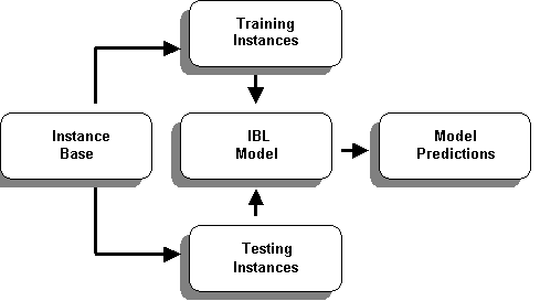
Figure 1. Structure of an IBL algorithm

The model shown in Figure 1 is a typical representation of IBL model in which the model predicts using instances from its instance base.

Types of IBL Algorithm

There are various types of IBL algorithm, which can build query-specific local models, which attempt to fit the training examples only in a region around the query point (Zhang et al., 1997).

Metric distance minimization (MDM)

MDM is perhaps the simplest instance-based learning method. In MDM, when a query is presented, the training example that is the closest to the query point, in terms of the Euclidean distance or some other suitable metric, is found out and that provides the parameters of that example as predicted output parameter.

K-nearest-neighbors (KNN)

KNN is a generalization of metric distance minimization. Instead of returning the parameters of the point that is most similar to the query point, KNN returns the average of the parameters of its (k) nearest neighbors, again defined in terms of Euclidean distance. A straightforward extension to this approach is distance-weighted nearest neighbors, in which instead of a straight average, we take a weighted average of the output parameters of the nearest neighbors, with the weight factor usually being the inverse of the distance from each neighbor to the query point.

K-surrounding-neighbors (KSN)

In the KSN algorithm (k) nearest neighbor are determined with the same formulae as of KNN algorithm. But the idea is to select the (k) instances in such a way that are not only close to the new instance, but also well distributed around the new instance. In other words, all selected instances should be close to new instance, but they should not be too close to each other. When selected instances are widely distributed around the new instance, more information is provided to derive the value of the new instance (Reich and Barai, 2000).

Criteria of Calculating the Nearest Neighbor

There are various methods by which the proximity of the new instance can be calculated (Zhang and Yang, 1998). The two methods used are given below:

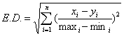
Similarity Index

In this method, the weight of an instance is its similarity to the new instance. The similarity is computed by the formula:

Where x = (x₁………….x_n) and y = (y₁…………y_n) are two instances,

n is the number of variables, and

max_i and min_i are the maximum and minimum values of the ith variables.

The value of the new instance x is calculated using the following formula:

Where w_i = similarity(x,i). i is the instance of the k selected instances, f_x is the value of x and f_i  is the value of the ith  selected instance.

Euclidean Distance

The normalized value of the new instance is calculated with respect to the instances in the Instance Base by the following formula:

where  max_i and min_i are the maximum and minimum values of the ith variables.

The main advantage of dividing the value of (x_i- y_i) by the difference of maximum and minimum value is that all the values are now in between 0 and 1 with proportionate weights according to nearness with the new instance.

Instance Based Learning Models Implementation

The implementation of Instance Based Learning model was done executing the programs written in MATLAB (Pratap, 2001).  The various IBL models are as follows

·        Model KNNC - K-nearest Neighbor by calculating similarity index

·        Model KSNC- K-surrounding Neighbor by calculating similarity index

·        Model KNNCNV- K-nearest Neighbor by calculating similarity index after normalizing the data set

·        Model KSNCNV- K-surrounding Neighbor by calculating similarity index after normalizing the data set

·        Model KNNED- K-nearest Neighbor by calculating Euclidean distance after normalizing the data set

Detail discussion about these models is given elsewhere (Agarwal, 2001).

Results and Discussion

In the present study, various IBL models were studied by varying the number of nearest neighbors, to determine the best IBL model and number of nearest neighbors required for the best performance. The success rates are summarized in a Tables 1-5.  All the models were found to provide same trend in the results.  

Table 1. Model KNNC - K-nearest Neighbor by calculating similarity index

Model	Input Variables	% Correct prediction of Neural Networks Model for Testing examples (Goh, 1996)	% Correct prediction by Model KNNC for Testing examples
			K-nearest Neighbors
			1	2	3	4	5	6
A4	M, qc1, t/s'0, D50	94	97	97	100	100	100	100
A5	M, qc1, s'0, a, t/s'0	86	91	91	97	97	97	97
A6	M, qc1, s'0, a, t/s'0,D50	94	100	100	100	100	97	97
A7	M, qc1, s0, s'0, a,t/s'0, D50	85	91	91	97	97	97	91
B5	M, qc1, s'0, a, D50	94	100	100	100	100	88	91

Table 2. KSNC- K-surrounding Neighbor by calculating similarity index  

Model	Input Variables	% Correct prediction of Neural Networks Model for Testing examples (Goh, 1996)	% Correct prediction by Model KSNC for Testing examples
			K-nearest Neighbors
			1	2	3	4	5	6
A4	M, qc1, t/s'0, D50	94	97	97	100	100	100	100
A5	M, qc1, s'0, a, t/s'0	86	91	91	97	97	97	97
A6	M, qc1, s'0, a, t/s'0,D50	94	100	100	100	100	97	97
A7	M, qc1, s0, s'0, a,t/s'0, D50	85	91	91	97	97	97	91
B5	M, qc1, s'0, a, D50	94	100	100	100	100	88	91

Table 3. Model KNNCNV- K-nearest Neighbor by calculating similarity index after normalizing the data set

Model	Input Variables	% Correct prediction of Neural Networks Model for Testing examples (Goh, 1996)	% Correct prediction by Model KNNCNV for Testing examples
			K-nearest Neighbors
			1	2	3	4	5	6
A4	M, qc1, t/s'0, D50	94	94	94	97	97	97	97
A5	M, qc1, s'0, a, t/s'0	86	94	94	97	97	97	97
A6	M, qc1, s'0, a, t/s'0,D50	94	100	100	97	97	97	97
A7	M, qc1, s0, s'0, a,t/s'0, D50	85	94	94	97	97	97	97
B5	M, qc1, s'0, a, D50	94	94	94	97	97	97	97

Table 4. Model KSNCNV- K-surrounding Neighbor by calculating similarity index after normalizing the data set

Model	Input Variables	% Correct prediction of Neural Networks Model for Testing examples (Goh, 1996)	% Correct prediction by Model KSNCNV for Testing examples
			K-nearest Neighbors
			1	2	3	4	5	6
A4	M, qc1, t/s'0, D50	94	97	97	100	100	100	100
A5	M, qc1, s'0, a, t/s'0	86	91	91	97	94	97	97
A6	M, qc1, s'0, a, t/s'0,D50	94	100	100	100	100	100	100
A7	M, qc1, s0, s'0, a,t/s'0, D50	85	91	91	97	97	97	97
B5	M, qc1, s'0, a, D50	94	100	100	100	100	100	100

Table 5. Model KNNED- K-nearest Neighbor by calculating Euclidean distance after normalizing the data set

Model	Input Variables	% Correct prediction of Neural Networks Model for Testing examples (Goh, 1996)	% Correct prediction by Model KNNED for Testing examples
			K-nearest Neighbors
			1	2	3	4	5	6
A4	M, qc1, t/s'0, D50	94	97	97	94	100	94	94
A5	M, qc1, s'0, a, t/s'0	86	94	94	97	97	97	97
A6	M, qc1, s'0, a, t/s'0,D50	94	97	97	97	97	97	97
A7	M, qc1, s0, s'0, a,t/s'0, D50	85	97	97	97	97	97	97
B5	M, qc1, s'0, a, D50	94	94	94	94	94	94	94

·        From Tables 1-5, it is observed that IBL models have performed much better than reported neural networks performance (Goh, 1996).

·        Similarity index based IBL models (Tables 1-4) have performed better than Euclidean distance based model (Table 5) for parameter combination of A6 and B5

·        Similarity index models for data without normalization, KNNC (Table 1) and KSNC  (Table 2), have demonstrated more or less equal performance.

·        Among similarity index models with normalized data, KNNCNV (Table 3) and KSNCNV (Table 4), K-surrounding neighbor based model has performed better than K -nearest neighbor model.

·        As a striking observation, it was found that parameters combination of B5 based model performed very well with surrounding nearest neighbors as 1-4 for similarity based models (Tables 2 and 4).

Based on the present study, following general observations have been made.

·        We have explored various Instance Based Learning (IBL) Models such as KNN and KSN with various kind of data modeling approaches for existing liquefaction potential assessment data of CPT. The results demonstrated that different modeling leads to better understanding of the dataset.

·        From the complete exercise, it was found the best IBL model in the present context could be KSN as it represents more realistic nature of capturing dataset behavior. IBL performance for assessment is satisfactory for the well-distributed set of data studied here.

·        KNN model gave the higher performance error in comparison to KSN model. The model is improved by introduction of surrounding neighbor model or the KSN model. For well-distributed set of data the results from the KNN and KSN models are comparable with results from the neural network model. 

·        The model performance was only checked with reported results of the literature and one needs to carry out some more parametric study and check the validity of the model with actual experimental data.

·        The proposed model always has to be tested before it is put into practice and hence there is a scope to check the model performance by carrying out some statistical evaluations such as resubstitution, hold-out and cross validation (Reich and Barai, 1999).

Summary

Liquefaction in the soil deposit causes huge damages to the property. So assessment of its potential is an important task to be carried out. Many models in the past have been used to do the work. In this paper, Instance Based Learning (IBL) is explored to assess the liquefaction potential. The performance of IBL was compared with reported neural networks based model and it was found that IBL performance better than neural networks model. Further the IBL models were studied with various kinds of nearest neighbor selection procedures and it was found that K - surrounding nearest neighbor based IBL model is well suited for well distributed data studied in this paper. Further to improve the model performance, it is worthwhile to explore the hybrid model combining IBL and neural networks. 

References

1. Agarwal, G. (2001), Instance based learning models for liquefaction potential assessment, B.Tech. Dissertation Report, Department of Civil Engineering, IIT Kharagpur, India.

2. Berrill, J. B., and Davis, R. O. (1985), "Energy dissipation and seismic liquefaction of sands: revised model", Soils and Foundation, Vol. 25, No. 2, pp: 106-118.

3. Christian, J. T., and Swiger, W. F. (1975), "Statistics of liquefaction and SPT results", Journal of Geotechnical Engineering Division, ASCE, Vol. 101, No. 11, pp: 1135-1150.

4. Goh, A.T.C. (1994), "Seismic liquefaction potential assessed by neural networks", Journal of Geotechnical Engineering, ASCE, Vol. 120, No. 9, pp: 1467-1480.

5. Goh, A.T.C. (1996),  "Neural network modeling of CPT seismic liquefaction data", Journal of Geotechnical Engineering, ASCE, Vol. 122, No. 1, pp: 70-73.

6. Kibler, D., Aha, D. and Albert, M. K. (1989), "Instance-based prediction of real values attributes", Computational Intelligence, Vol. 5, pp: 51-58.

7. Law, K. T., Cao, Y. L., and He, G. N. (1990), "An energy approach for assessing seismic liquefaction potential", Canadian Geotechnical Journal, Vol. 27, pp: 320-329.

8. Liao, S. S. C., Veneziano, D. and Whitman, R. V. (1988), " Regression models for evaluating liquefaction probability", Journal of Geotechnical Engineering, ASCE, Vol. 114, No. 4, pp: 389-411.

9. Pinto, P. S. (1999), Earthquake Geotechnical Engineering, Proceedings of the Second International Conference on Earthquake Geotechnical Engineering, Lisbon, Portugal, A A Balkema.

10. Pratap, R. (2001), Getting Started With MATLAB Version 6: A Quick Introduction for Scientists and Engineers, Oxford Press.

11. Reich, Y. and Barai, S. V. (1999), "Evaluating machine learning models for engineering problems", Artificial Intelligence in Engineering, Vol.13, pp: 257-272

12. Reich, Y.  and Barai S V (2000), " A methodology for building neural networks models from empirical engineering data", Engineering Applications of Artificial Intelligence, Vol. 13, No. 6, pp: 685-694.

13. Seed, H. B., Tokimatsu, H., Harder, L. F., and Chung, R. M. (1985), "Influence of SPT procedure in seismic liquefaction resistance evaluations", Journal of Geotechnical Engineering, ASCE, Vol. 111, No. 2, pp: 1425-1445.

14. Tokimatsu, K. and Yoshimi, Y., (1983), "Empirical Correlation of Soil liquefaction based on SPT N-value and fine content", Soils and Foundation, Vol. 23, No. 4, pp: 56-74.

15. Tung, A. T. Y., Wang, Y. Y. and Wong, F. S. (1993), "Assessment of liquefaction potential using neural networks" Soil Dynamics and Earthquake Engineering, Vol. 12, pp: 325-335.

16. Ural, D. N. and Saka, H. (1998),  "Liquefaction assessment by artificial neural networks", The Electronic Journal of Geotechnical Engineering, Vol. 3, 1998.

17. Zhang, J., and Yang, J. (1998), An application of instance –based learning to highway accident frequency prediction, Department of Computer Science, Utah State University, Logan UT 84322-4205  - A Technical Report.

18. Zhang, J., and Yim, Y. S., and Yang, J., (1997), "Intelligent selection of instance for prediction functions in lazy learning", Artificial Intelligence Review, Kluwer Academic Publishers.

	© 2002 ejge